Generic Vectors

TODO: intro

After reading these notes you should be able to:

TODO: learning objectives

Lists

Last chapter, we discussed atomic vectors. Importantly, we learned that atomic vectors have a type, and each element of an atomic vector must have the same type.

c(1, 2, 42)

[1]  1  2 42

Using the c() function here, we are combining three length one atomic vectors with type double, which is allowed, and thus produces a length three atomic vector of type double.

typeof(c(1, 2, 42))

[1] "double"

We also saw that if we attempt to create a vector by combining vectors of different types, R will simply force them to all have the same type.

c(42, TRUE, "foo")

[1] "42"   "TRUE" "foo"

typeof(c(42, TRUE, "foo"))

[1] "character"

Does R have the ability to store a collection of objects that do not have the same type? Yes. Vectors can do this, in particular generic vectors which are most often called lists. Like all vectors, they are simply a collection of elements (which are objects) but unlike atomic vectors, the individual elements may have different types. Atomic vectors are homogeneous objets, whereas lists are heterogeneous objects.

To create a list, we can use a very similar looking syntax, that is, replacing c() with list().¹

list(42, TRUE, "foo")

[[1]]
[1] 42

[[2]]
[1] TRUE

[[3]]
[1] "foo"

typeof(list(42, TRUE, "foo"))

[1] "list"

First, note that this object that we have created has type list. Because the elements to longer all have the same type, clearly we need a new type for this object.

Note that the c() function can actually be used to create lists. If an object passed to c() is of type list, c() will return a list, as list is higher in the the coercion hierarchy than any of the atomic vector types. The full hierarchy is: NULL < raw < logical < integer < double < complex < character < list < expression. We’ve now seen everything except expression.

c(list(1), 1)

[[1]]
[1] 1

[[2]]
[1] 1

typeof(c(list(1), 1))

[1] "list"

Next, note that the way a list prints is different than an atomic vector. Generally, an atomic vector only gives you occasional notes about the index of each element.

100:1

  [1] 100  99  98  97  96  95  94  93  92  91  90  89  88  87  86  85  84  83
 [19]  82  81  80  79  78  77  76  75  74  73  72  71  70  69  68  67  66  65
 [37]  64  63  62  61  60  59  58  57  56  55  54  53  52  51  50  49  48  47
 [55]  46  45  44  43  42  41  40  39  38  37  36  35  34  33  32  31  30  29
 [73]  28  27  26  25  24  23  22  21  20  19  18  17  16  15  14  13  12  11
 [91]  10   9   8   7   6   5   4   3   2   1

Lists, if they do not have named elements, state each index in double brackets, for example, [[2]].

list(42, TRUE, "foo")

[[1]]
[1] 42

[[2]]
[1] TRUE

[[3]]
[1] "foo"

The single brackets you see, in particular each [1] is not part of the printing of a list, but instead, the printing of the atomic vectors that are stored within the elements of the list.

Like, atomic vectors, we can name the elements of a list as we create it.

list(a = 42, b = TRUE, c = "foo")

$a
[1] 42

$b
[1] TRUE

$c
[1] "foo"

Here, the name of each element is shown preceded by the $ operator which we will discuss shortly. Again, the [1] that you see are printed based on the atomic vectors stored in each element.

Let’s create a few objects and assign them names so we can continue to discuss.

foo = list(42, TRUE, "foo")
bar = list(a = 1:10,
           b = "Hello, World!",
           c = log,
           d = list(a = 1, b = "z"))
baz = c(4, 3, 2, 1)

For comparison, we’ve created three objects and assigned them the names foo, bar, and baz.

foo

[[1]]
[1] 42

[[2]]
[1] TRUE

[[3]]
[1] "foo"

Here we see that foo references a list with unnamed elements.

bar

$a
 [1]  1  2  3  4  5  6  7  8  9 10

$b
[1] "Hello, World!"

$c
function (x, base = exp(1))  .Primitive("log")

$d
$d$a
[1] 1

$d$b
[1] "z"

Like foo, bar also references a list, but with named elements.

Lastly, baz refers to an atomic vector of type double.

First, recall that both atomic vectors and lists (generic vectors) are vectors². We can verify this with the is.vector() function.

c(is.vector(foo), is.vector(bar), is.vector(baz))

[1] TRUE TRUE TRUE

To be sure which is an atomic vector or list, we can use the is.atomic() and is.list() functions.

c(is.atomic(foo), is.atomic(bar), is.atomic(baz))

[1] FALSE FALSE  TRUE

c(is.list(foo), is.list(bar), is.list(baz))

[1]  TRUE  TRUE FALSE

You might have noticed a couple interesting objects stored in bar, in particular a function³ and another list. Lists allow us to store objects of any type. Because of the ability to store lists within lists, you may hear lists referred to as recursive vectors.

Don’t be fooled by the potential recursive nature of lists, they are still a one-dimensional object like an atomic vector. As such, they have a length equal to the number of elements.

c(length(foo), length(bar), length(baz))

[1] 3 4 4

Sometimes, the printing of a list, especially larger lists that you will encounter in practice, can be a bit unwieldy. As such, it is often easy to instead look at the structure of a list with the str() function.

str(bar)

List of 4
 $ a: int [1:10] 1 2 3 4 5 6 7 8 9 10
 $ b: chr "Hello, World!"
 $ c:function (x, base = exp(1))  
 $ d:List of 2
  ..$ a: num 1
  ..$ b: chr "z"

Here, we see a wealth of information:

This object is a list, of length four.
The first element, named a, is an integer vector of length ten.
The second element, named b, is an character vector of length one.
The third element, named c, is a function!
The fourth element, named d, is a list of length two!
- The first element of this list, named a is a numeric (double) vector of length one.
- The first element of this list, named b is a character vector of length one.

This information can also be found in the RStudio environment panel.

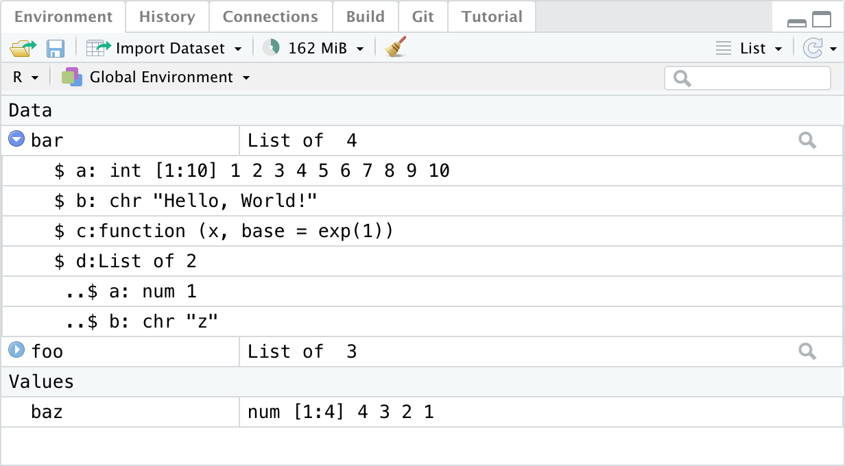
Clicking the arrow filled blue circle for an object of type list will reveal the same information provided by the str() function. Additionally, clicking the magnifying glass will reveal a more in-depth RStudio specific object viewer. This viewer can also be accessed using the View() function.

View(bar)

Occasionally, you may want to force a list to be an atomic vector. This can be done with the unlist() function.

unlist(foo)

[1] "42"   "TRUE" "foo"

Note that here, there is obviously coercion that necessarily must take place. Also, be aware, that sometimes unlist() will fail to produce an atomic vector if it contains element that simply cannot be placed in an atomic vector, like a function.⁴

Extracting Elements

Like atomic vectors, we can extract elements of a generic vector. We’ll continue to delay subsetting in general a bit longer, but introduce some new syntax that is needed to extract a single element of a generic vector.

Before we move to generic vectors, recall that extracting an element from an atomic vector will result in a object of length one, which is the same type as the vector you’re doing the extraction from.

typeof(baz)

[1] "double"

baz[2]

[1] 3

typeof(baz[3])

[1] "double"

Obviously, this won’t always be the case with list. With lists, when we extract a particular element, it could be an object of any type.

To extract a single element from a list, you can use either the double bracket operator, [[, or the dollar sign operator, $.

The double bracket can be used to extract an element by its index.

foo

[[1]]
[1] 42

[[2]]
[1] TRUE

[[3]]
[1] "foo"

foo[[2]]

[1] TRUE

Note that using a single bracket, [, would do something very, very different.

foo[2]

[[1]]
[1] TRUE

Notice, this is a list. More on this when we discuss subsetting in general.

If a list has named elements, you can use either the double bracket or dollar sign operator.

bar[["b"]]

[1] "Hello, World!"

bar$b

[1] "Hello, World!"

Note that, after we extract an object, we can go right ahead and use said object. For example, remember that we stored the log() function. We can extract and use if.

bar$c(c(1, 2, 3))

[1] 0.0000000 0.6931472 1.0986123

Data Frames

Data frames are lists with some additional restrictions. They are perhaps the most useful object for performing data analysis.

Let’s start by making a list.

list(
  a = 5:1,
  b = rep("a", times = 5),
  c = c(TRUE, FALSE, TRUE, FALSE, TRUE),
  d = c(1, 1, 1, 1, 1)
)

$a
[1] 5 4 3 2 1

$b
[1] "a" "a" "a" "a" "a"

$c
[1]  TRUE FALSE  TRUE FALSE  TRUE

$d
[1] 1 1 1 1 1

When creating this list, we were somewhat careful with the objects used to populate the list. In particular, notice that each object has the same length.

A data frame, when used for data analysis, can often be thought of as observations and variables, which we generally associate with rows and columns. But clearly, the above output does not invoke rows and columns to the reader. Enter the data frame.

To create a data frame, we use similar syntax to a list, but with the data.frame function.

data.frame(
  a = 5:1,
  b = rep("a", times = 5),
  c = c(TRUE, FALSE, TRUE, FALSE, TRUE),
  d = c(1, 1, 1, 1, 1)
)

  a b     c d
1 5 a  TRUE 1
2 4 a FALSE 1
3 3 a  TRUE 1
4 2 a FALSE 1
5 1 a  TRUE 1

Notice, when this object prints, the rows and columns become abundantly clear.

A data frame is a list where each element is a vector, each with the same length.⁵ The vast majority of the time, each vector is atomic, but that is not always the case.⁶

Let’s give this data frame a name.⁷

some_df = data.frame(
  a = 5:1,
  b = rep("a", times = 5),
  c = c(TRUE, FALSE, TRUE, FALSE, TRUE),
  d = c(1, 1, 1, 1, 1)
)

some_df

  a b     c d
1 5 a  TRUE 1
2 4 a FALSE 1
3 3 a  TRUE 1
4 2 a FALSE 1
5 1 a  TRUE 1

Note that both the rows and columns have names. They are not actually part of the object. They are only names, an attribute. The column names are actually just the names of the elements, since a data frame is a list. The row names are an additional attribute.

attributes(some_df)

$names
[1] "a" "b" "c" "d"

$class
[1] "data.frame"

$row.names
[1] 1 2 3 4 5

names(some_df)

[1] "a" "b" "c" "d"

colnames(some_df)

[1] "a" "b" "c" "d"

rownames(some_df)

[1] "1" "2" "3" "4" "5"

Notice an additional attribute, class. More on this later.

We can verify that data frames are indeed lists.

is.list(some_df)

[1] TRUE

Also note that it is a data frame.

is.data.frame(some_df)

[1] TRUE

But the previous lists we saw are indeed not data frames.

is.data.frame(foo)

[1] FALSE

Like lists, you eventually deal with large data frames in practice, and printing them becomes tedious. You should instead check their structure.

str(some_df)

'data.frame':   5 obs. of  4 variables:
 $ a: int  5 4 3 2 1
 $ b: chr  "a" "a" "a" "a" ...
 $ c: logi  TRUE FALSE TRUE FALSE TRUE
 $ d: num  1 1 1 1 1

Again, this information can be found in RStudio’s environment panel. Additionally, RStudio has a data frame viewer which can be incredibly useful.

View(some_df)

Like atomic vectors, when you create data frames, you may run into vector recycling.

data.frame(
  a = 5:1,
  b = "a",
  c = c(TRUE, FALSE, TRUE, FALSE, TRUE),
  d = 1
)

  a b     c d
1 5 a  TRUE 1
2 4 a FALSE 1
3 3 a  TRUE 1
4 2 a FALSE 1
5 1 a  TRUE 1

However, thankfully, with data frames, it only allows recycling of compatible lengths.

data.frame(
  a = 5:1,
  b = "a",
  c = c(TRUE, FALSE),
  d = 1
)

Error in data.frame(a = 5:1, b = "a", c = c(TRUE, FALSE), d = 1) : 
  arguments imply differing number of rows: 5, 1, 2

Because a data frame is a list, which is a vector, they have a length.

length(some_df)

[1] 4

We can obtain the number of rows with the nrow() function.

nrow(some_df)

[1] 5

We can also obtain the number of columns with the ncol() function. But recall, this is also the length, because a data frame is a vector, in particular, a list.

ncol(some_df)

[1] 4

To simultaneously obtain the number of rows and columns, as a double vector of length two, use the dim() function.

dim(some_df)

[1] 5 4

Unlike lists and atomic vectors, data frames require unique names. If you attempt to create a data frame without unique names, R will change them.

data.frame(a = 1, a = 2)

  a a.1
1 1   2

In practice, you will need to create data frames, but even more often, you will read pre-existing files, often stored with comma separated values, into R as a data frame for processing, manipulation, and analysis. Later, we’ll discuss function such as read.csv() that provide this functionality.

Extracting Elements

typeof(some_df)

[1] "list"

Remember, a data frame is a list. So extracting elements (columns) uses the same syntax.

some_df

  a b     c d
1 5 a  TRUE 1
2 4 a FALSE 1
3 3 a  TRUE 1
4 2 a FALSE 1
5 1 a  TRUE 1

some_df[[2]]

[1] "a" "a" "a" "a" "a"

some_df[["c"]]

[1]  TRUE FALSE  TRUE FALSE  TRUE

some_df$d

[1] 1 1 1 1 1

Each of the above extracts the atomic vector contained in the element (by name or number) of the data frame.

Again, we’re using either the double bracket operator, [[, or the dollar sign operator, $. The single bracket, [, performs a very different operation which we will explore in the next chapter.

Summary

TODO: You’ve learned to…

What’s Next?

TODO: subsetting

TODO

TODO: probably don’t use partial matching. when can you use partial matching?

Footnotes

The c() function can also create lists, if one of the objects that you’re combining is a list, due to coercion.↩︎
Often, you will simply hear an object referred to as a vector, without qualification. Often, from context this may be understand to imply an atomic vector.↩︎
Functions have type closure.↩︎
This is because functions, unlike most objects, are not vectors. Try: is.vector(log)↩︎
More technically, it is a list with attributes for names, row.names, and has class data.frame.↩︎
Also, creating vectors with columns that are lists is a bit more difficult to accomplish.↩︎
We suggest avoiding naming data frames df. You’ll see this often, but it can lead to confusion as there is already a function named df in your environment when you load R. (It is the distribution function for an F distribution.) This will help you avoid the infamous error message: Error in df$a : object of type 'closure' is not subsettable. Note: When you inevitably see this error message, replace “closure” with “function” when you read it and the meaning will be much cleared. You can’t subset a function.↩︎