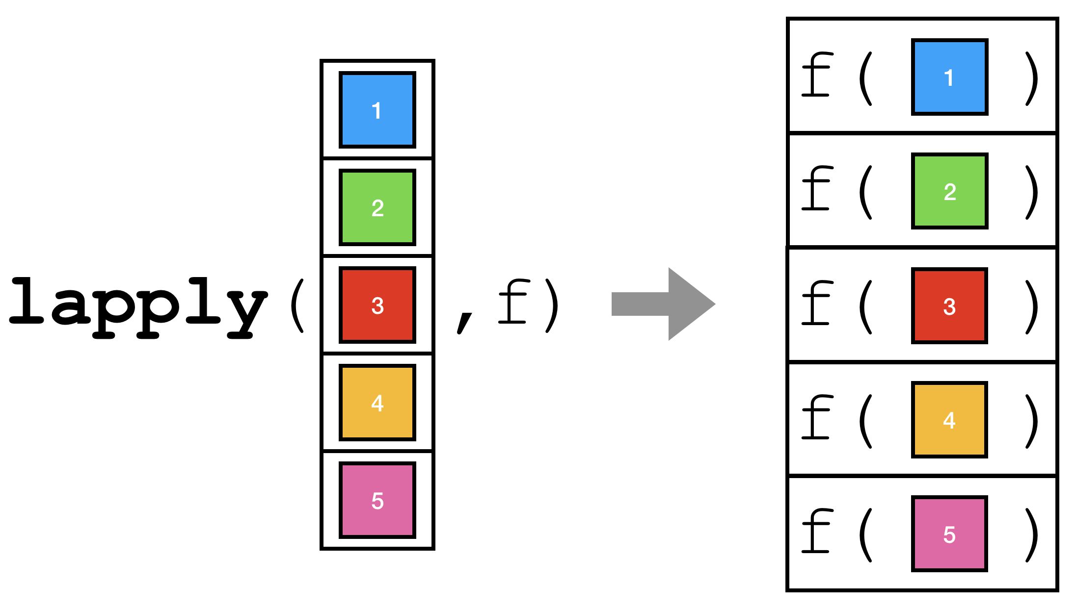
lapply(X = some_list, FUN = f)Iteration
In programming, iteration is the act of repeating a set of instructions. This can be done several different ways:
- Repeat until some condition is met.
- Repeat a certain number of times.
- Repeat through elements of a vector.
In R, the last example here, repeating through elements of a vector, is by far the most common. Because of this, R has built-in functions that make this type of iteration extremely easy. While R does provide the usual iteration abilities through the use of for and while loops, these should not be your go-to methods for performing iteration.
After reading these notes you should be able to:
- TODO: learning objectives
Apply Functions
One of the most common operations that you will encounter while programming with R is running a function with each element of some vector as input and collecting the results in a vector.
lapply.lapply
The function in R that performs the operation described above is lapply. The general syntax is:
That is, some_list is a vector (atomic vector or list) that the function f will be “applied” to each element of. Note that it is customary to not name the arguments to lapply.
lapply(some_list, f)Let’s start with a very simple example.
lapply(1:3, log)[[1]]
[1] 0
[[2]]
[1] 0.6931472
[[3]]
[1] 1.098612Here we see the log function applied to each of the elements of the vector 1:3. This would be the same as running the following:
list(
  log(1),
  log(2),
  log(3)
)
[[1]]
[1] 0
[[2]]
[1] 0.6931472
[[3]]
[1] 1.098612Clearly, this isn’t a particularly useful example, as we could simply do the following:
log(1:3)[1] 0.0000000 0.6931472 1.0986123Although, note that lapply is returning a list, but the above returns an atomic vector. More on that in a moment.
For now, know that lapply will return a list that has the same length as the input vector.1
Let’s look at an example of iterating over a list.
set.seed(42)
ex_list = list(a = runif(5),
               b = runif(5),
c = runif(5))ex_list$a
[1] 0.9148060 0.9370754 0.2861395 0.8304476 0.6417455
$b
[1] 0.5190959 0.7365883 0.1346666 0.6569923 0.7050648
$c
[1] 0.4577418 0.7191123 0.9346722 0.2554288 0.4622928lapply(ex_list, max)$a
[1] 0.9370754
$b
[1] 0.7365883
$c
[1] 0.9346722Again, here the input was a list of length three, so the output is as well. You might wish the output was an atomic vector. Again, more on that soon.
lapply(ex_list, range)$a
[1] 0.2861395 0.9370754
$b
[1] 0.1346666 0.7365883
$c
[1] 0.2554288 0.9346722Finally, a slightly more useful example. This returns the same object as the following:
list(
  range(ex_list[[1]]),
  range(ex_list[[2]]),
  range(ex_list[[3]])
)
[[1]]
[1] 0.2861395 0.9370754
[[2]]
[1] 0.1346666 0.7365883
[[3]]
[1] 0.2554288 0.9346722Hopefully, it is becoming clear that lapply can be used to write concise, useful, and readable code.
What if we want to use a function with more than one argument? For example:
multiply_and_power = function(x, c, p) {
  c * x ^ p
}multiply_and_power(x = 2, c = 3, p = 0.5)[1] 4.242641multiply_and_power(x = 2, c = 1:3, p = 0.5)[1] 1.414214 2.828427 4.242641Be aware that depending on how we specify the values we pass to the arguments, there is likely going to be some length coercion taking place.
To use this function together with lapply, we simply add the values of the additional parameters as arguments to lapply.2
lapply(1:3, multiply_and_power, c = 1:5, p = 2)[[1]]
[1] 1 2 3 4 5
[[2]]
[1] 4 8 12 16 20
[[3]]
[1] 9 18 27 36 45What did this code do?
list(
  multiply_and_power(x = 1, c = 1:5, p = 2),
  multiply_and_power(x = 2, c = 1:5, p = 2),
  multiply_and_power(x = 3, c = 1:5, p = 2)
)
[[1]]
[1] 1 2 3 4 5
[[2]]
[1] 4 8 12 16 20
[[3]]
[1] 9 18 27 36 45What if we wanted to iterate over a different argument, say c instead of x? Specify x and p in the call to lapply. Now lapply will iterate over c.
lapply(1:3, multiply_and_power, x = 1:5, p = 2)[[1]]
[1] 1 4 9 16 25
[[2]]
[1] 2 8 18 32 50
[[3]]
[1] 3 12 27 48 75So, this time, we did the following:
list(
  multiply_and_power(x = 1:5, c = 1, p = 2),
  multiply_and_power(x = 1:5, c = 2, p = 2),
  multiply_and_power(x = 1:5, c = 3, p = 2)
)
[[1]]
[1] 1 4 9 16 25
[[2]]
[1] 2 8 18 32 50
[[3]]
[1] 3 12 27 48 75Sure, you could simply use this instead, but imagine needed to iterate over 1:100000 instead.
sapply
Let’s return to the example that found the maximum of each element of a list.
set.seed(42)
ex_list = list(a = runif(5),
               b = runif(5),
c = runif(5))lapply(ex_list, max)$a
[1] 0.9370754
$b
[1] 0.7365883
$c
[1] 0.9346722As expected, the result is a list. However, notice that each element of said list is an atomic vector of length one, of the same type. We could actually check that using lapply.
lapply(lapply(ex_list, max), typeof)$a
[1] "double"
$b
[1] "double"
$c
[1] "double"lapply(lapply(ex_list, max), length)$a
[1] 1
$b
[1] 1
$c
[1] 1It probably seems like what we really want as output here is an atomic vector that is the same length as the input vector. We can obtain this result by switching from lapply to sapply.
sapply(ex_list, max) a b c
0.9370754 0.7365883 0.9346722 The “S” in sapply refers to the simplifying action taken by the function. Much of the details of how the simplification works follows the usual rules of the coercion hierarchy. It is probably best not to worry too much about these rules, and not rely on simplification too much. Generally, it is probably best to use sapply in the case we’ve just seen here: you are certain the result of the function applied to each element is an atomic vector of length one, each with the same type.
Another example:
sapply(1:3, log)[1] 0.0000000 0.6931472 1.0986123But again, this example isn’t truly necessary, as the following is even better:
log(1:3)[1] 0.0000000 0.6931472 1.0986123We show this to demonstrate that many operations in R are already vectorized, so there is no need to iterate.
Other Apply Functions
Other apply functions exist. Many are rarely used. One that might be of interest is vapply which will do simplification like sapply, but the user will need to specify the expected outcome of each iteration, which will make the simplification more predictable.
vapply(1:3, log, double(1))[1] 0.0000000 0.6931472 1.0986123vapply(1:3, log, integer(1))Error in vapply(1:3, log, integer(1)) : values must be type 'integer',
but FUN(X[[1]]) result is type 'double'
Another that you will likely see is the apply function. We would advise avoiding this unless you truly understand what it does. Also, beware, it should probably not be used with data frames.3
Later we will look at an alternative solution to the apply function through the use of the purrr package.
Loops
Loops are another form of control flow. Essentially, they allow you to explicitly specify the repetition of some code, in contrast to the apply functions above that did so explicitly.
Welcome to R Club.
- The first rule of R Club is: Do not use
forloops!- The second rule of R Club is: Do not use
forloops!- And the third and final rule: If you have to use a
forloop, do not grow vectors!— Unknown
Loops are very common in programming, however, in R, it is best to avoid them unless you truly need them. The general hueristic you should use to determine if you need a loop or apply function is:
- Use a loop when the result of the next iteration depends on the result of the previous iteration.
- Use an apply function when the results of each iteration are independent.4
for
The most common looping structure is a for loop. The generic syntax is:
for (element in vector) {
  code_to_run
}
We’ll refer to element as the loop variable.
Let’s look at a specific example.
x = double(length = 5)
for (i in 1:5) {
  x[i] = i ^ 2
}
x
[1] 1 4 9 16 25First, note that for is not a function, which is why you should consider placing a space between it and the parenthesis that follows. Next, (i in 1:5) is considered the header of the loop which defines how the iteration will take place. Here the name of the loop variable is i. The code inside the braces, {} is called the body of the loop, much like the body of a function.
- Each time through the loop,
i, will take one of the values from1:5. Or generally, the loop variable will take the value of each element of a vector. - For each value of
i, the codex[i] = i ^ 2will run. In general, for each value of the looping variable, the code in the body will run. And often, that code will depend on the looping variable, like we see here.
So, the above for loop ran each of the following:
x[1] = 1 ^ 2
x[2] = 2 ^ 2
x[3] = 3 ^ 2
x[4] = 4 ^ 2
x[5] = 5 ^ 2
This should make it clear that the purpose of a loop is to repeat code, without actually having to repeatedly type it.
As has become a theme, this for loop is truly useless in R. We could have simply done:
(1:5) ^ 2[1] 1 4 9 16 25Here, i is functioning much like the name of a function argument, except now, we pass a new value, an element of 1:5, each time through the loop.
You can use any name you want for the loop variable, but i, j, and k are most common.
for (some_long_var_name in 1:5) {
  print(some_long_var_name)
}
[1] 1
[1] 2
[1] 3
[1] 4
[1] 5A for loop is a very powerful structure, so it will not be possible for us to illustrate all possible usage examples.
Let’s look at a correct loop written poorly, then the same loop written better, and try to draw some conclusion about best practices with for loops.
Before proceeding, let’s introduce the seq_along function.
seq_along(5:1)[1] 1 2 3 4 5Essentially, seq_along returns the indexes of a vector. Or, you could think of it as returning the result of the following:
1:length(5:1)[1] 1 2 3 4 5Let’s use a for loop to create a sequence of numbers. The first two numbers will be 10, and 5. Elements after that will be calculated as:
\[ x_i = 3 \cdot \frac{x_{i - 1}}{x_{i - 2}} \]
We’ll use a loop to create a sequence of length ten that follows this specification.
First, a bad example of how to write a loop to accomplish this:
for (i in 1:10) {
  if (i == 1) {
    x = 10
  } else if (i == 2) {
    x = c(x, 5)
  } else {
    x = c(x, 3 * x[i - 1] / x[i - 2])
  }
}
x
[1] 10.0 5.0 1.5 0.9 1.8 6.0 10.0 5.0 1.5 0.9We see the correct resulting vector, x, but we have used some sub-optimal technique. In particular, we “grew” the x vector. The use of x = c(x, some_new_element) takes what was x, then creates a new x but combining the previous x with some new element. Do not do this. This is one of the reasons people incorrectly think R is slow. This operation is slow, but there is no need for it.
Instead, let’s pre-allocate the x which we will store our results in.
x = double(10) # pre-allocate x to be a double vector of the correct length
for (i in seq_along(x)) {
  if (i == 1) {
    x[i] = 10
  } else if (i == 2) {
    x[i] = 5
  } else {
    x[i] = 3 * x[i - 1] / x[i - 2]
  }
}
x
[1] 10.0 5.0 1.5 0.9 1.8 6.0 10.0 5.0 1.5 0.9This time, since x already existed, we are simply replacing individual elements of an already existing vector. This is faster. Any time you grow or add new elements (that is you increase the length of a vector) there is a copy operation taking place under the hood that you could have avoided.
Also, by pre-allocating x, we can now use seq_along(x). In some applications we might be creating x with a program, and we wouldn’t know its length ahead of time!
Some general ideas to keep in mind:
- Do not attempt to iterate over and store results in the same vector.
- Pre-allocate a “results” vector and update individual elements as you progress through the loop. Do not grow vectors.
- Use
seq_alongand iterate over indexes rather than elements of a vector.
We’ve already discussed why the second item is a problem. Let’s now create an example that demonstrate items one and three.
The following function will check if an number is even.
is_even = function(x) {
  x %% 2 == 0
}
We also create a vector y that stores some numbers.
set.seed(42)
y = sample(1:10, size = 20, replace = TRUE)
y
[1] 1 5 1 9 10 4 2 10 1 8 7 4 9 5 4 10 2 3 9 9Our goal is to create a logical vector, the same length as y, containing TRUE at any index where y is even.
This will, not work:
for (i in y) {
  y[i] = is_even(i)
}
To better see the issue, temporarily place a print() statement inside the loop.
set.seed(42)
y = sample(1:10, size = 20, replace = TRUE)
for (i in y) {
  print(i)
  y[i] = is_even(i)
}
[1] 1
[1] 5
[1] 1
[1] 9
[1] 10
[1] 4
[1] 2
[1] 10
[1] 1
[1] 8
[1] 7
[1] 4
[1] 9
[1] 5
[1] 4
[1] 10
[1] 2
[1] 3
[1] 9
[1] 9y [1] 0 1 0 1 0 4 0 1 0 1 7 4 9 5 4 10 2 3 9 9So i takes values from y, but by doing so, we don’t have access to the indexes at which we need to replace with the result of is_even. Let’s use seq_along.
set.seed(42)
y = sample(1:10, size = 20, replace = TRUE)
for (i in seq_along(y)) {
  y[i] = is_even(y[i])
}
y
[1] 0 0 0 0 1 1 1 1 0 1 0 1 0 0 1 1 1 0 0 0Note that inside of i, we now need to change i to y[i] to get the value rather than the index each time through the loop.
But there’s still an issue! We have 0 and 1 instead of FALSE and TRUE. Coercion!
set.seed(42)
y = sample(1:10, size = 20, replace = TRUE)
res = logical(length(y))
for (i in seq_along(y)) {
  res[i] = is_even(y[i])
}
res
[1] FALSE FALSE FALSE FALSE TRUE TRUE TRUE TRUE FALSE TRUE FALSE TRUE
[13] FALSE FALSE TRUE TRUE TRUE FALSE FALSE FALSEMuch better. But again, remember, many things in R are vectorized:
is_even(y) [1] FALSE FALSE FALSE FALSE TRUE TRUE TRUE TRUE FALSE TRUE FALSE TRUE
[13] FALSE FALSE TRUE TRUE TRUE FALSE FALSE FALSEThis example did not need a loop, because results from one iteration to the next were independent. In the previous example, this was not the case, and was an example of when you truly need a loop.
Note that these examples have used atomic vectors, but, not reason we couldn’t use a list!
while
A while loop will repeat code until some condition is no longer met. The general syntax is:
while (condition) {
  code_to_run
}
Let’s see an example.
x = 10
y = double(length = 10)
while (x > 0) {
  print(x)
  y[x] = x ^ 2
  x = x - 1
}
[1] 10
[1] 9
[1] 8
[1] 7
[1] 6
[1] 5
[1] 4
[1] 3
[1] 2
[1] 1x[1] 0y [1] 1 4 9 16 25 36 49 64 81 100Here, the loop runs until x is no longer greater than 0.
Notice, that if we don’t modify x inside the loop, it could run forever! An infinite loop!5
You’ll see for loop more often, but while loops are useful when you don’t know how many iterations you’ll need ahead of time, but instead have a stopping condition.
x = 1
while(x > 1e-10) {
  print(x)
  x = x / 2
}
repeat
- TODO: not very important, ignore for now.
- TODO: next, break
Summary
- TODO: You’ve learned to…
What’s Next?
- TODO: ?
Footnotes
Think l for list. Although, it is unclear if that is the etymology of the name of the
lapplyfunction.↩︎If you check the documentation for
lapply, you’ll notice an argument called.... More on this later, but this is what allows R to pass these additional arguments to the function.↩︎The
applyfunction is useful when working with matrix objects, which we have been avoiding.↩︎Also check that you can’t just use a vectorized operation.↩︎
If you experience an infinite loop, use Ctrl + C in the console to escape it. Or press the stop button.↩︎